Artificial Intelligence is such a broad term that people struggle to know the starting point. I remember myself being there . Getting the concept of what is Artificial Intelligence , what is Machine Learning , what is Deep Learning and what is Reinforcement Learning were the few challenges I faced. All I had back then were knowledge of few programming languages and curiosity to explore.
What is Artificial Intelligence?
It’s kind of nothing but a term used to define a branch of computer science which explains simulation of intelligence by machines.
What Is Machine Learning ?
Before getting into machine learning let’s focus on traditional programming. So in traditional programming we give Input (data we provide),define set of rules or constraints and machine gives us output(what we wanted). In Machine Learning we give machine/program Input(data) and output(what we want) and tell machine/program to figure out the rules for us.
Still not clear?
Basically what traditional programming looks like:
If we want to know a given number is odd or even we do is
INPUT:
a = int(input("Enter a number"))
Algorithm / Processing:
if (a % 2) != 0:
   print("the number is odd")
else:
   print ("the number is even")
Here we gave machine/program an input to work on and wrote some constraints i.e. if the number is divisible by 2 or not and if the remainder is not 0 then give output as odd otherwise even.
Similarly In machine learning we give machine/programs a set of data and their actual output that we know and tell the machine to figure out how can you(machine) map the given data so that next time when I give data with unknown output, you(machine) should be able to give me relevant output without high randomness .
How can this be achieved?
A simple way to demonstrate machine learning is with Linear Regression. Here we will be looking at regression with single variable . Multivariate Linear Regression is the topic for next discussion.
Single Variable Linear Regression
Before getting into the core part , first lets discuss what is this term Regression . So In Machine Learning there are various techniques that we can apply to given data depending upon the problem domain.
For example : If we wanna predict the price of a house from given data which includes size of the house , no of bedrooms then it is a regression problem . Which means we need the machine to predict continuous value (i.e price of the house)
There are more than regression under machine learning techniques. Like
Classification : Here the output is what category does the given data falls under like recognizing hand written digits , output will always falls under (0–9) since there are only 10 classes that a digit can be classified or represented.
Clustering , Association , Anomaly detection , sequence mining , Dimension reduction , Recommendation system and so on.
Things Required :
- Python, pandas, numpy , matplotlib installed on your system
- Basic python programming and mathematics()
Lets Get Started
Basic understanding of mathematics is sufficient for now since we will be dealing with only one variable.
y = mx + c
Here:
y is a dependent variable
x is some variable
m is the slope
c is the y intercept (0,c)
so linear regression works on the same principle as the equation for a straight line. After all it gives us an imaginary line which fits best to our data .We will be referring this same terminology in a different way. A more standard approach. Since we want out machine to learn m and c we will be referring to them with Theta.
So our equation becomes:
y = Theta(0) * X(0) + Theta(1) * X(1) .......... equation(1)
How they became 4 terms?
y = m * x + 1 * c
Here, we consider c as Theta(0) and m as Theta(1). In previous equation the 4th term was present but hidden. As you can see there was 1 multiplying c. The same concept applies here. Theta(0) consist of only ones hence multiplying something with one will always give you the same number. We arrange such(Theta) variable in (n,1) dimensional vector. Here n refers to the no of features or in simple way the no of columns in training data or the number of Thetas we want machine to calculate.
What Is scalar , vector , matrix , tensors?
scalar is just a number e.g 2 , 3 , 1
vectors are one dimensional array. e.g [1,2,3]
matrix are arrays having 2 dimensions. e.g [[1,2],[2,2]]
tensors are n dimensional arrays where n > 2
Back to the equation(1)
So in Machine Learning we call them as hypothesis. For now consider this as a linear function that give output by multiplying a vector and a matrix with (n,m) dimension.
Code
def hypothesis(theta, X):
    return np.dot(X, theta)
Explanation
So we define a function hypothesis that takes two parameters and returns the dot product or matrix(X) and a vector(theta). Nothing magical here.
Loss Function
You may have question that how do we know machine is learning ? A machine could predict number randomly right? Wrong . We check the loss function , if the loss is conversing down to minimum then we consider it good . General theory is that when you plot loss with respect to number of iteration the figure should be a convex . So how can this be calculated ?
There are wide range of loss functions for simplicity we will mean squared error (mse) or simply we calculate the sum of square of differences. How do we do that .
Code
def cost(theta, X, y):
    pred = hypothesis(theta, X)
    constant = 1 / (2 * m)
    delta = pred - y
    J = constant * np.sum(delta ** 2)
    return J
Explanation
Here we calculate the prediction or the output given by the hypothesis function .
pred = hypothesis(theta, X)
So there can’t be mean without dividing the output with the number of quantities or data. Right? Same thing here:
constant = 1 / (2 * m)
So till now we have covered the mean part . Now where is the error part.
delta = pred - y
error are just the difference between the prediction made by machine and the actual output. We represent our actual output as y.
Now the squared part:
np.sum(delta ** 2)
We just calculate the square of errors.
Combining this all (mean , squared and error):
J = constant * np.sum(delta ** 2)
So that’s why we call them mean squared errors
Gradient (The Learning Part)
This is the part where theta is manipulated . We predict , calculate the difference between predicted output and actual output and finally update the learned theta.
Code
def gradient_descent(theta, X, y, alpha=0.01):
    cost_his = []
    theta_his = []
    for i in range(epochs):
        temp_theta = theta
        J = cost(theta, X, y)
        cost_his.append(J)

        for j in range(theta.shape[0]):
            if j == 0:
                temp_theta[j] = theta[j] - (alpha / m) * np.sum(hypothesis(theta, X) - y)
            else:
                temp_theta[j] = theta[j] - (alpha / m) * np.sum((hypothesis(theta, X) - y) * X[:, 1].reshape((m, 1)))

        theta = temp_theta
    return theta, theta_his, cost_his
Explanation
Here, there are some terms newly introduce like alpha, epoch.
alpha: It is the learning rate or the pace at which the machine learns the parameters. If the learning rate is too high the gradient might oscillate and never reach the global minimum and if the learning rate is too low then the gradient converge too slow.
epoch: The number of iterations you want the machine to learn on. Hyperparameters tuning are topics for future discussions. For now they are the number of repetition you want your machine to train.
for i in range(epochs):
        temp_theta = theta
        J = cost(theta, X, y)
        cost_his.append(J)
Here we define a loop for 0 to (epochs-1) times. We assign theta to a temporary variable because we don’t want to manipulate theta directly. Then we calculate the cost and append it to a list. Nothing much going here.
for j in range(theta.shape[0]):
   if j == 0:
      temp_theta[j] = theta[j] - (alpha / m) * np.sum(hypothesis(theta, X) - y)
         else:
temp_theta[j] = theta[j] - (alpha / m) *
np.sum((hypothesis(theta, X) - y) * X[:, 1].reshape((m, 1)))
This is the most important part. Here we define a loop for n times where n is the number of features and m is the no of training data.
n = no of columns in training data(excluding y )
m = number of rows in training data
Basically what it is doing in this conditional is that for theta(0) don’t multiply it with the input or training data. You can find various approaches where only the else part is sufficient. But for better understanding lets divide them so that for theta(0) we don’t multiply with the column 1’s only.
temp_theta[j] = theta[j] - (alpha / m) * np.sum(hypothesis(theta, X) - y)
Here we are updating theta[i] by subtracting the product of learning rate and the gradient.
temp_theta[j] = theta[j] - (alpha / m) * np.sum((hypothesis(theta, X)
- y) * X[:, 1].reshape((m, 1)))
You may wonder why are we using theta[j] - gradient * learning rate. To make you more clear lets take an example when your machine predicts greater than the actual output.
since all the outputs predicted by our machine is higher that means (hypothesis(theta, X) - y) is positive . The sum of positive number is also positive. That means our theta is too large and is predicting greater results. To make it converge or make accurate prediction we want our machine to reduce the theta so theta[j] - (alpha / m) * np.sum((hypothesis(theta, X) - y) * X[:, 1].reshape((m, 1))) reduces the theta.
Same concept applies when the output or prediction made by our machine is lower. Since all the outputs predicted by our machine is lower that means (hypothesis(theta, X) - y) is negative. Adding up negative number always gives us negative number . This means our theta is too low . To get more accurate results we need to add up or increase some value to theta. This is done with the same equation. We know multiplying negative to negative gives us positive result. So the negative in the formula and the negative output creates positive output and hence the theta gets increased .
Combining all the concept
def hypothesis(theta, X):
    return np.dot(X, theta)


def cost(theta, X, y):
    pred = hypothesis(theta, X)
    constant = 1 / (2 * m)
    delta = pred - y
    J = constant * np.sum(delta ** 2)
    return J


def gradient_descent(theta, X, y, alpha=0.01):
    cost_his = []
    theta_his = []
    for i in range(epochs):
        temp_theta = theta
        J = cost(theta, X, y)
        cost_his.append(J)
        for j in range(theta.shape[0]):
            if j == 0:
                temp_theta[j] = theta[j] - (alpha / m) * np.sum(hypothesis(theta, X) - y)
            else:
                temp_theta[j] = theta[j] - (alpha / m) * np.sum((hypothesis(theta, X) - y) * X[:, 1].reshape((m, 1)))
        theta = temp_theta
    return theta, theta_his, cost_his
Problem Solving With Linear Regression (Single Variable)
Getting the dataset : Click Here
Importing required libraries
import pandas as pd
import numpy as np
import matplotlib.pyplot as plt
Reading data using pandas
data = pd.read_csv('data.csv')
Data pre-processing (i.e changing data into more usable format)
X = np.array(data["X"])
X = X.reshape((X.shape[0], 1))
X = np.insert(X, 0, 1, axis=1)
y = np.array(data["Y"])
y = y.reshape((y.shape[0], 1))
print("shape of y ", y.shape)
print("Shape of X", X.shape)
Output
Shape of X (97, 2)
shape of y  (97, 1)
Defining the algorithm
def hypothesis(theta, X):
    return np.dot(X, theta)


def cost(theta, X, y):
    pred = hypothesis(theta, X)

    constant = 1 / (2 * m)

    delta = pred - y

    J = constant * np.sum(delta ** 2)
    return J


def gradient_descent(theta, X, y, alpha=0.01):
    cost_his = []
    theta_his = []
    for i in range(epochs):
        temp_theta = theta
        J = cost(theta, X, y)
        cost_his.append(J)

        for j in range(theta.shape[0]):
            if j == 0:
                temp_theta[j] = theta[j] - (alpha / m) * np.sum(hypothesis(theta, X) - y)
            else:
                temp_theta[j] = theta[j] - (alpha / m) * np.sum((hypothesis(theta, X) - y) * X[:, 1].reshape((m, 1)))

        theta = temp_theta
    return theta, theta_his, cost_his
def prediction(theta, X):
    return theta[0] + X * theta[1]
Defining some constants
m = y.shape[0]
epochs = 10000
Running the algorithm
initial_theta = np.zeros((X.shape[1], 1))
theta, theta_his, cost_his = gradient_descent(initial_theta, X, y, 0.001)
Predicting Values
preds = prediction(theta, X[:, 1])
Plotting the predicted values
plt.plot(X[:, 1], preds)
plt.show()
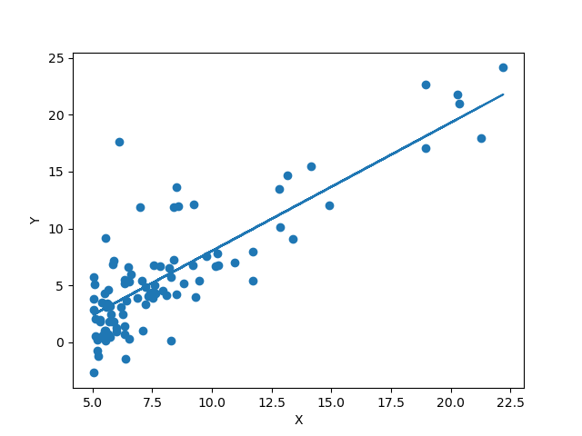
Linear Regression
Conclusion:
We can see that our algorithm fits fine but there are various ways we can make it better. That will be covered on upcoming posts.
So summarizing we saw what is machine learning, how does machine learning really work and Linear Regression with single variable.